Bayesian Optimization

Opening Discussion

Levels of Optimization Problem Solving

In general, we can divided the way to solve optmization problem into $3$ levels:

Level 0: Non-derivative, including some familiar approaches such as: Grid Search, Random Search, Bayesian Optimization, etc.
- Pros: Fast computation, do not require the function to be smooth, i.e. no differentiable required, the function need continous
- Cons: It is heuristic, not a theory-based method
Level 1: First-derivative. $∇f(x) = f(x_i)_i$. The most popular one is Gradient Descent (Adam, Nesterov, etc.)
- Pros: Efficient to converge in local minimum/maximum
- Cons: Computational since it requires backpropagation
Level 2: Second-derivatie. $J(f) = f(x_i, x_j)_{ij}$ (i.e. Newton)
- Pros: Very effective, faster convergence than level-1 method
- Cons: Significantly compuational

Bayesian Optimization is the one in level 0

Bayesian Optimization

When to use Bayesian Optimization

Supose that we are optimzing a function $f(x, \Theta)$ $\max_{\Theta}f(x,\Theta)$

We can consider Bayesian Optimzation if $f$ satisfy following conditions:

$f$ has to be continuous
$f$ is expensive to evaluate
$f$ is a blackbox. In other words, we don’t know characteristic of $f$ (convex, non-convex, derivative, etc.)

Fundementals of Bayesian Optmization

Instead of directly optimizing $f$, we approximate it by other easier evaluation function $P$, and define a strategy $u$ to optimize $P$

$P$ - Surrogate model:
- the alternative of $f$, easier to optmize
- Gaussian Process, etc.
$u$ - Acquisition function:
- strategy to optmize surrogate model
- Expected Improvement (EI), Upper Condidence Bound (UCB), etc.

In this article, we focus on the most popular surrogate model - the Gaussian Process

Gaussian Process

As mentioned, $f$ is black box and expensive to evaluate. Hence, the surrogate model should be an alternative that is easier to evaluate. A good intuition is to approximate $f$ as a distribution (normally Gaussian Distribution).
In other words, we consider $f$ as a Gaussian Distribution with mean $\mu(x)$ and standard deviation $\sigma^2(x)$

\[f(x) \sim \mathcal{N}(\mu(x), \sigma^2(x))\]

Hence, the Gaussian Process $P$ has the Probability Density Function (PDF) as

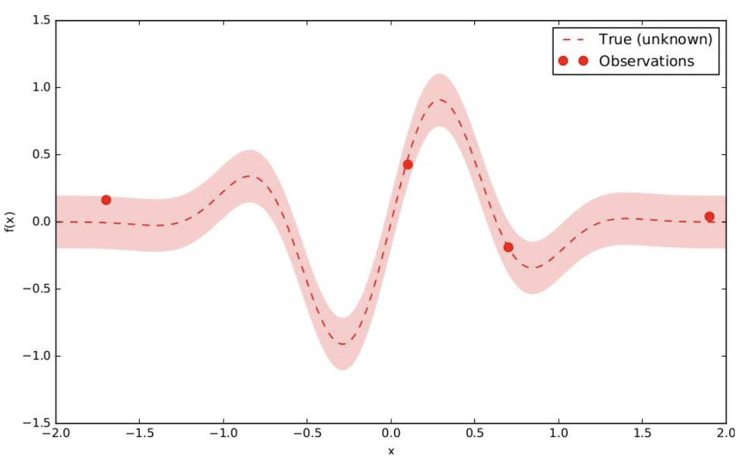
\[P(f(x)=y) = \frac{1}{\sqrt{2\pi\sigma^2}} \exp{\frac{|y - \mu(x)|^2}{2\sigma^2}}\]

The figure below demonstrates it as a distribution approximation

Therefore, Gaussian Process makes use of Bayes Theory. Since we literally has no information about how $f$ looks like (the solid red line), we just has some initial observations (blue circle). The surrogate model gives us a probabilistic estimation of $f$ as a distribution (the area limited by dash red line)

From this, we need to select the next point (i.e. $x_+$) to sample from $f$. The strategy to select the next point from the observation of surrogate model is taken by acquisition function.

After the next point is sampled, i.e. $\{x_+, y=f(x_+)\}$. We continue to fit it as prior knowledge to surrogate model and continue to select next point, i.e. $x_{++}$. Gradually, we will have a more knowledge on how $f$ looks like as the belief keeps increasing.

Acquisition function

The strategy that proposes the next sampling point is decided by acquisition function $u$. Particularly, we optimize $u$ over surrogate model $P$. Note that as mentioned, those functions are easier to optimize comparing to $f$
There are lots of acquisition function, the most popular ones are Expected Improvement $EI$, and Upper Confidence Bound $UCB$. In this article, we define $EI$ as the acquisition function.

Expected Improvement function is defined as $EI(x) = \mathbb{E} \max (x - f(x^*))$

The intuition is that the chosen next sampling point should have maximal expected values comparing the best of those from observations. The best point from existing observations is denoted as $x^* = \arg\max_{x_i \in D} f(x_i)$

Since we are optimizing acquisition function over a Gaussian Process, the more particular formula can be clarified as $EI(x) = \begin{cases} \displaystyle (\mu(x) - f(x^*) - \xi)\varphi(Z) + \sigma(x)\phi(Z) & \text{if} & \sigma(x) > 0 \\ \displaystyle 0 & \text{if} & \sigma(x) = 0 \end{cases}$

where

\[Z = \begin{cases} \displaystyle \frac{\mu(x) - f(x^*) - \xi}{\sigma(x)} & \text{if} & \sigma(x) > 0 \\ \displaystyle 0 & \text{if} & \sigma(x) = 0 \end{cases}\]

The adjusted parameter $\xi$ is use to balance between exploitation and exploration of two summation terms in the above equation, respectively.

High $\xi$ means we lower the probability of first term (the one calculating with mean $\mu$, i.e. the certainty), hence, increase the probability of second term (the one calculating with variance $\sigma$, i.e. the uncertainty) –> we want to explore on the area of uncertainty more, and vice versa.

The complete process

In summary, the overall process of Bayesian Optimization can be clarified as follows: We want to find the optimal values of objective function $f$ with surrogate model $P$ and acquisition function $u$. Initially, we have limited observations $D={x_N, y_N}$. The iteration below is how Bayesian Optimization works:
—
1. Fit ${x_N, y_N}$ to approximate surrogate model $P$
2. Optimize acquisition function $u$ over $P$ to sample the next point $x_{N+} = u(x)$
3. Evaluate $\{x_{N+}\}$ on $f$ to get $y_{N+}$
4. Add $\{x_{N+}, y_{N+}\}$ to D and repeat the process

The detail about implementation from scratch can be found at [4]

Below is the demonstration step-by-step:

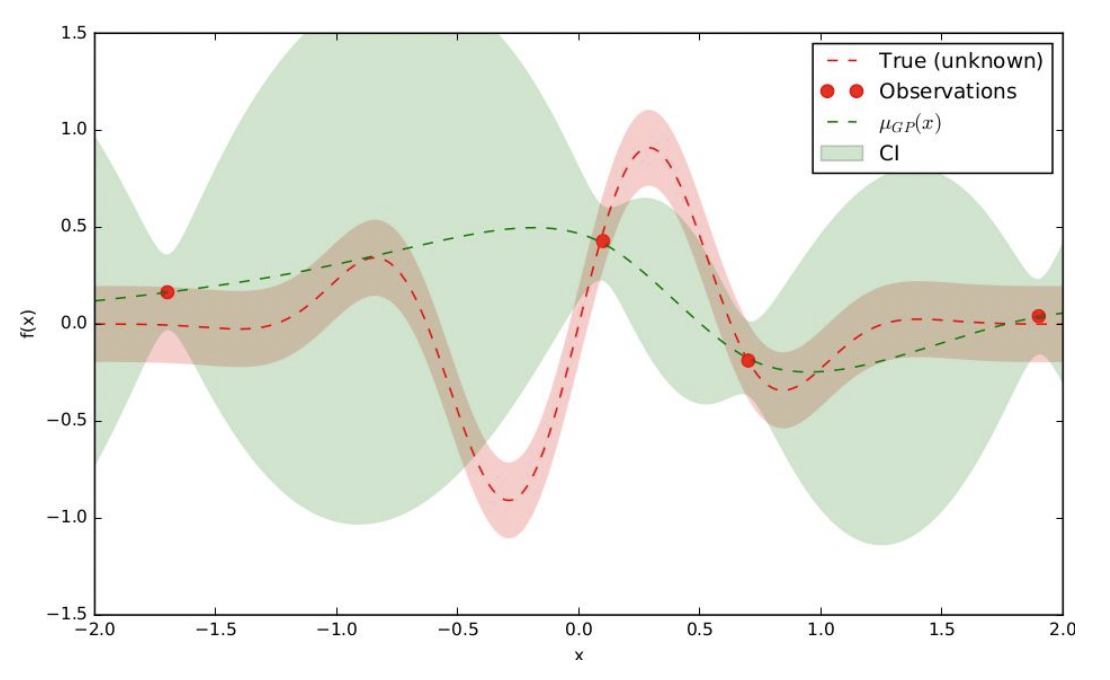
Suppose we want to find the values that maximize the objective function below (which is unknown) with some initial observations.

Approximate a surrogate model $P$ (i.e. Gaussian Process). The green area is CI - Confidence Interval drawn from $\sigma^2$ of surrogate model, depicts the uncertainty over objective function

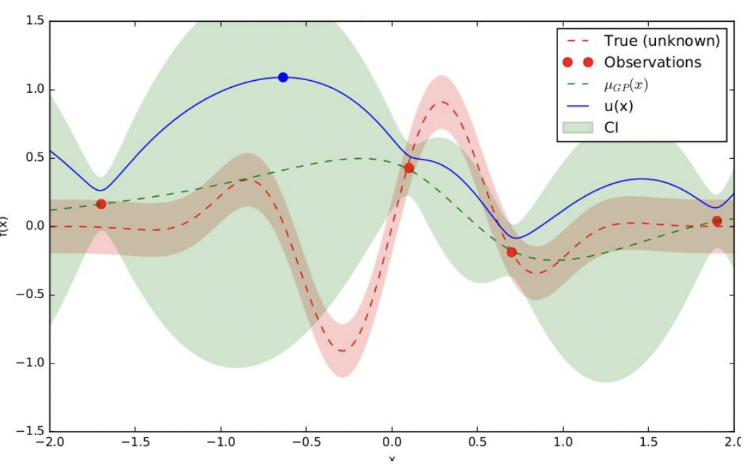
Apply acquisition function $u$ over $P$. As a result, it proposed the next sampling point as blue circle

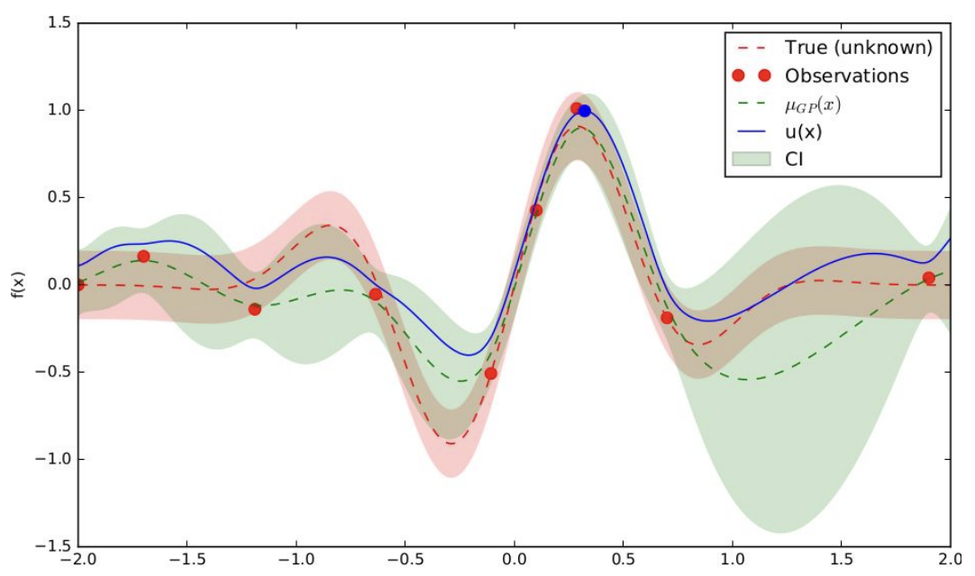
Evaluate the proposed sampling point using objective function. We can observe that the uncertainty significantly narrow down. We repeat this process through a number of iterations

Discussion:

We may have a general observation about Bayesian Optimization. However, there are still some that we have resolve yet:

Alternatively, we optimize acquisition function over surrogate model instead of objective function since it cheaper, yet it is not clear the approach to optimize acquisition function
Beside Expected Improvement, other popular acquisition functions are UCB, Probability of Improvement

Implementation

To simplify the implementation, we suppose that:

We have already known the objective function for the verification.
The surrogate model makes use of Gaussian Process Regression provided by scikit-learn
The process of optimizing the acquisition function will be handled by scipy employing Broyden–Fletcher–Goldfarb–Shanno algorithm[6]

We will implement

The Bayesian Optimization process
A method maximizing acquisition function
An instance of acquisition function, i.e. Expected Improvement

Set up

# TO-DO: problem with scipy > 1.4, find out solution

!pip unistall scipy --y
!pip install scipy==1.4.1

import numpy as np
import matplotlib.pyplot as plt

# assume the objective function f
def f(X, noise=0.):
    return -np.sin(6*X) - X**2 + 0.05*X + noise * np.random.randn(*X.shape)

# Initial samples
noise=0.2
X_inits = np.array([[-0.9], [1.1]])
y_inits = f(X_inits, noise)

print(X_inits.shape, y_inits.shape)

# Bounds of x
bounds = np.array([[-1.0, 2.0]])

(2, 1) (2, 1)

# enrich samples to draw objective function
X = np.arange(bounds[:,0], bounds[:,1], 0.01).reshape(-1,1)
y = f(X,noise=0)

print('The objective function and initial observations: ')
plt.figure(figsize=(12,8))
plt.plot(X, y, 'y--', lw=2, label='Objective function')
plt.plot(X, f(X, noise), 'gx', lw=1, alpha=0.2, label='Noisy samples')
plt.plot(X_inits, y_inits, 'kx', mew=3, label='Initial samples')
plt.legend()
plt.show()

The objective function and initial observations: